Energy Musings, August 31, 2021

Energy Musings contains articles and analyses dealing with important issues and developments within the energy industry, including historical perspective, with potentially significant implications for executives planning their companies’ future. While published every two weeks, events and travel may alter that schedule. I welcome your comments and observations. Allen Brooks

Download the newsletter

August 31, 2021

Climate Science Is Simple, Highly Complex, And Confusing
CO₂ is our enemy. It is heating the world, yet significantly greening the planet and increasing harvests. Understanding climate science is challenging. It is not settled, and it is complex. We trace the history of climate science into the modern era. The role of carbon is highlighted, plus its role in driving climate change. Unfortunately, this is a long read. READ MORE

EVs Are In The News But Not Always In The Best Light
EV sales have roared ahead this year globally, but they still represent a miniscule share of the world fleet. GM’s Bolt recall is a financial disaster. Mark Mills explores EV carbon legacy. READ MORE

Fossil Fuels’ Death Prediction May Be Premature
Heading toward COP26 means calls for ending fossil fuels. The problem is that around the world we are seeing governments resort to more coal generation to keep the lights on. Why? READ MORE

Climate Science Is Simple, Highly Complex, And Confusing

“In the spring I have counted one hundred and thirty-six different kinds of weather inside of four and twenty hours.” That was Samuel L. Clemons, aka Mark Twain, a resident of Hartford, Connecticut, speaking at the New England Society’s 71^st Annual Dinner on December 22, 1876, at Delmonico’s restaurant in New York City. Clemons was known for his witty observations about the variability of New England weather. He once wrote, “Climate is what we expect, weather is what we get.”

“Everybody talks about the weather, but nobody does anything about it,” is often attributed to Clemons, but he didn’t say it. Rather co-author Charles Dudley Warner, with whom he wrote the novel The Gilded Age, said it. Today, we are fortunate to have a global organization, the International Panel on Climate Change (IPCC), trying to do something about our climate and our weather. Its latest report tells us how bad our climate is, but a path exists to avoid the worst of the disasters predicted by climate models if we act now to choke off burning fossil fuels.

From the days of the ancient Greeks, people believed humans could alter temperatures and influence rainfall by chopping down trees, plowing fields, or irrigating deserts. Over time, these beliefs were disabused, with the last one that “rain follows the plow’ dying with the Dust Bowl of the 1930s.

The science of climate change emerged two hundred years ago when a French scientist, Joseph Fourier, calculated that Earth was so far from the Sun that its climate should be colder unless some other factor was keeping it warm beyond the incoming sunlight. He postulated that the energy from the Sun in the form of visible and ultra-violet light (known back then as “luminous heat”) could easily pass through the Earth’s atmosphere and heat up the planet’s surface. Because the “non-luminous heat” (now known as infrared radiation) emitted by the Earth’s surface could not leave as readily, he reasoned the atmosphere was acting as an insulating blanket. Developing this idea further was stymied by the lack of detailed measurement tools.

Exhibit 1. Chart Of Climate Science Milestones And Scientists Responsible

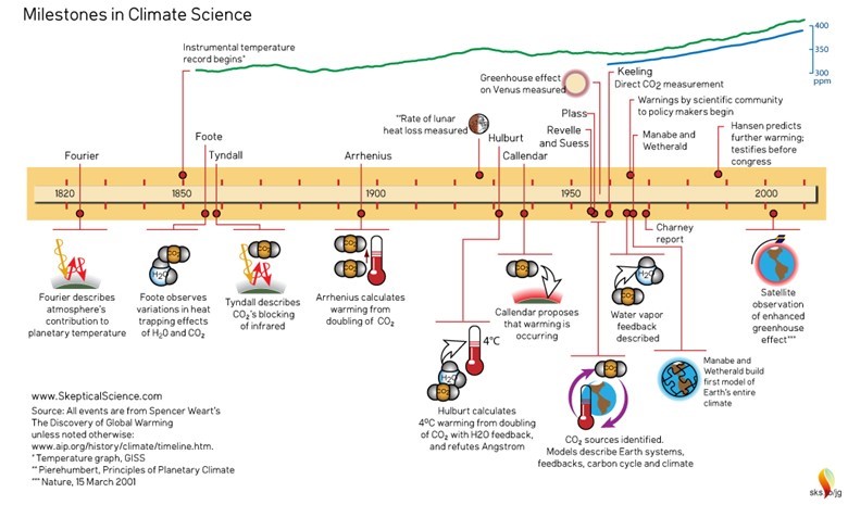
Source: SkepticalScience.com

Roughly 35 years later, American scientist Eunice Foote observed the variations in heat trapping effects of water vapor and carbon dioxide (CO₂). As we wrote in our last Energy Musings:

More recently, it is thought that American scientist Eunice Foote made a similar discovery in 1856, three years before Tyndall. Her experiment was crude, and it is possible she did not comprehend what exactly she had measured or whether she understood its significance. She did not differentiate between heat from the whole solar spectrum and what we now call long-wave infrared, which is responsible for the greenhouse effect. Nevertheless, her experiments did provide evidence of the absorption of heat by CO₂ and moist air.

Awareness of Foote’s experiment was not well known until Irish scientist John Tyndall’s experiments were heralded a few years later. This was despite Foote’s experiment being discussed in a research paper and at a scientific organization’s annual meeting. Again, from our article:

In 1859, the Irish physicist John Tyndall conducted an experiment at the Royal Institution in London that confirmed the existence of the greenhouse gas effect of our atmosphere. He demonstrated the absorption and radiation by certain gases in what we now call long-wave infrared radiation. Tyndall wrote: “Thus the atmosphere admits of the entrance of solar heat; but checks its exit, and the result is a tendency to accumulate heat at the surface of the planet.” While Tyndall acknowledged the work of Joseph Fourier in 1824 and Claude Pouillet in 1836 who had identified the rudimentary principles underlying the greenhouse gas effect on our atmosphere, what he had done was to detect and explain the physical basis of the greenhouse process and identify the gases responsible.

Tyndall’s work was an important milestone for the greenhouse gas explanation for the warming of the planet. His contemporaneous drawings of his experiments, as well as observations about them from his private and public lectures helped to understand what he had discovered. It was that water vapor was the strongest absorber of radiant heat in the atmosphere and is the principal gas controlling the Earth’s surface temperature. He noted that without water vapor, the Earth’s surface would be “held fast in the iron grip of frost.” The absorption by other gases such as CO₂, CH₄, nitrogen, oxygen, and ozone existed but was relatively small.

Tyndall’s drawings of his experiment led other scientists to question some of his conclusions, and whether his observations were distorted by issues with his equipment. An example was that the length of the tube could distort the experiment’s conclusions – a shorter one leads to increased concentrations of the gas within the tube compared to the atmosphere.

Exhibit 2. Drawing Of Tyndall’s Experiment Proving Greenhouse Gas Effect

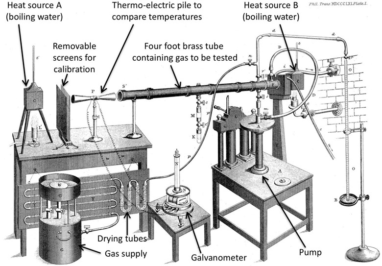
Source: ecojesuit.com

Apparently, Tyndall had no knowledge of Foote’s experiments, or he ignored them, even though they were reported in leading scientific journals. What was significant, however, was those two scientists, separated by the Atlantic Ocean, reached similar conclusions about various gases trapping heat, as well as how changes in their concentration would cause changes in the global temperature. Fournier’s “insulating blanket” had been confirmed and its components identified. The question was whether the most important component was water vapor or CO₂.

 

The answers came from other scientists who advanced the evolution of the greenhouse gas theory. In 1896, Svante Arrhenius wondered what the cooling effect would be if CO₂ in the atmosphere were cut in half? His question came from wondering how to explain past ice ages and whether volcanic activity might have contributed to lowering the temperature. His calculations showed that such a CO₂ cut would reduce temperatures by about 1.5º C (2.7º F). His curiosity led him to calculate the impact from a doubling of CO₂, which indicated a 1.6º C (2.9º F) increase.

Arrhenius’ calculations were met with skepticism, primarily because they were seen to be too simple. Another Swede, Knut Ångström, questioned them and conducted his own experiment. He found that when CO₂ was reduced by a third, there was little temperature change, which led him to conclude that the absorption bands of the light spectrum at which CO₂ is absorbed were quickly saturated so the absorption would not increase. The analysis was complicated by the fact water vapor also absorbs infrared radiation, and due to the quality of the instruments available, the absorption bands of the two gases overlapped one another. Thus, increasing CO₂ would be unable to absorb more infrared radiation in the spectrum bands where more abundant water vapor was already blocking.

With better instruments, the reported absorption-decrease due to a one-third cut in CO₂ turned out to be 2.5-times what Ångström calculated, sufficient to alter the global temperature. It was further discovered that even though the upper levels of the atmosphere were unsaturated by CO₂, they still could retain the heat. But, at the time, Ångström’s calculations were considered correct and Arrhenius’ wrong.

The climate change topic paused for about 35 years. Then, English engineer Guy Callendar revisited the actual levels of CO₂ in the atmosphere and compared them to the warming temperature record of the early 20^th century. He found CO₂ levels had increased by about 10%. As he investigated various other aspects of the atmosphere and CO₂, he prepared his own calculations of what could happen to global temperatures with rising amounts of CO₂. His calculation suggested a 2º C (3.6º F) warming from a doubling of CO₂.

Climate research increased after World War II with the beginning of the nuclear age. The advent of computers gave scientists more power to analyze temperature and climate data. In 1956, physicist Gilbert Plass examined the warming from increasing CO₂, which he published in the paper “The Carbon Dioxide Theory of Climatic Change” in the journal Tellus. It confirmed that a doubling of CO₂ would warm the climate by 3º-4º C (5.4º – 7.2º F). He further postulated that at the rate of mid-1950s carbon emissions, the planet would warm by 1.1º C (2º F) by the end of the century.

The nuclear age also introduced research into carbon isotopes, as ¹⁴C was released by nuclear explosions. ¹⁴C is an unstable carbon isotope that has six protons and eight neutrons in the nuclei of its atoms. The most abundant carbon isotope is ¹²C that has six protons and six neutrons. ¹⁴C is subject to radioactive decay, which allows its radioactivity to be tracked as it moves around in the atmosphere. The research into ¹⁴C led to the understanding that long-lived gases in the atmosphere were well-mixed throughout the layers, and from pole to pole.

¹⁴C has a short half-life, which is why radiocarbon dating is only used for estimating the lives of recent things and not ancient ones. In coal and crude oil, all the ¹⁴C has been decayed away, so burning them only releases non-radioactive ¹²C and the stable ¹³C. It was shown from an examination of the carbon isotopes in trees that the younger the wood, the more ¹²C and ¹³C there was relative to ¹⁴C. This was the fingerprint of burning fossil fuels contributing to global warming.

In 1958, the Scripps Institution of Oceanography installed a monitoring station on top of Hawaii’s Mauna Loa Observatory. Scripps’ geochemist Charles Keeling was instrumental in securing the funding for the monitoring observatory and in outlining how to record CO₂ levels. Thus, the chart produced from the observatory’s record of CO₂ concentrations in the atmosphere is known as the Keeling Curve. Because the Hawaii location is in the middle of the Pacific Ocean, away from possible polluting areas, it is considered representative of the carbon concentration for the global atmosphere.

Exhibit 3. Keeling Curve Shows Steady Rise In CO₂ Concentration In Atmosphere

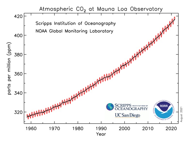
Source: NOAA

Estimates are that by burning fossil fuels representing carbon previously buried deep underground, we are adding each year about 4.5% of the annual flow of the natural carbon cycle. According to scientist Steven Koonin, the author of Unsettled: What Climate Science Tells Us, What It Doesn’t, And Why It Matters, when Earth was formed 4.5 billion years ago it had a fixed endowment of carbon. That carbon is found in different places, referred to as “reservoirs.” The largest reservoir is Earth’s crust, which contains most of the carbon, estimated at 1.9 billion gigatons (Gt). The second largest deposit, about 40,000 Gt, is found in the oceans, primarily the deep oceans. About 2,100 Gt is stored in soils and living things, and 5,000-10,000 Gt in fossil fuels. The approximate 850 Gt of carbon in the atmosphere, primarily as CO₂, is about 25% of the carbon at or near Earth’s surface (soils, plants, and shallow ocean), but only 2% of the total carbon in the oceans.

When examining the Keeling Curve above, note how it fluctuates during each year. That is the Earth “breathing.” It represents the seasonal flow of roughly 25% of Earth’s carbon moving from one natural reservoir to another. This volume is moving due to photosynthesis, in which plants turn atmospheric CO₂ into organic matter and then returns the carbon to the atmosphere through plant respiration and as organic matter decays. The Mauna Loa seasonal fluctuations represent the Northern Hemisphere breathing because it has the largest land mass. A benefit of the rise in atmospheric CO₂ has been the “greening” of the planet, documented by studying satellite images of Earth over time. The chart below shows how leaf areas have grown or shrunk over 1982-2015, which documents the greening that more CO₂ has produced.

Exhibit 4. The Greening Of Earth Due To Rise In Atmospheric CO₂

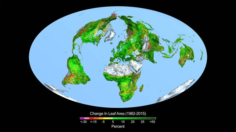
Source: NASA: Credits: Boston University/R. Myneni

There is little question that the rise in CO₂ has been due to human activities for the past 150 years. There are many measures that support this conclusion. One of the more recent was the discovery that over the past thirty years there has been a detectable and steady decrease in the atmosphere’s oxygen concentration. The decrease roughly matches what was needed to turn fossil carbon into CO₂.

Although most of the major theories about why Earth’s global climate warmed and cooled over the last million years was formed by the early 1900s, it wasn’t until the 1970s that scientists began pulling all the pieces together into a holistic approach to explain how the climate system functioned. In the early 1970s, the global cooling that was evident from the 1950s onward shifted the focus onto why the average temperature anomaly was negative. Falling temperatures were occurring despite rising CO₂ levels, which should have been driving temperatures higher. NASA scientists modeled the effects of pollution in the form of aerosols and sulfur emissions in the atmosphere and concluded that a significant increase in these pollutants could lead to a cooling phase. Scientists began examining the climate data and some postulated that it was possible the interglacial warming phase the world was in was ending and it was heading into a new Ice Age. Cleaning up the atmosphere by eliminating the production of ozone-depleting chemicals, also known as chlorofluorocarbons, led to a resumption of warming, which seemed to end the idea of a new Ice Age ahead.

About this time, a new climate tool emerged – ice cores ‒ for demonstrating that CO₂ had driven temperatures up in the past. If it had happened regularly in past glacial cycles, it must be happening today, was the view. This proof would be substantiation of the greenhouse effect.

The first known attempt to drill an ice core was conducted by Louis Agassiz in 1840 on the Unteraargletscher in the Swiss Alps. One hole reached a depth of 20 feet and another eight feet. By the late 1890s, several expeditions had drilled cores in Greenland. Perfecting the technology to drill ice cores took decades, as scientists drilled on glaciers and ice sheets in many locations around the world. The primary targets were Greenland and Antarctic.

Exhibit 5. A Chuck Of An Ice Core

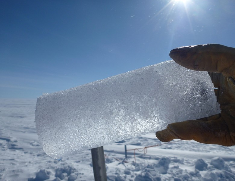
Source: climate.gov

Ice cores contain minute bubbles of prehistoric air trapped by snow that eventually became layers of ice. Once an ice core is extracted, these bubbles can be isolated and analyzed in a vacuum. They provide information about the composition of past atmospheres, through ice ages and interglacial periods. We have learned that during the frozen depths of the last ice age, CO₂ levels in the atmosphere were much lower than today – around 200 parts per million. In the mid-1980s, the famous Vostock core was drilled to a depth of two kilometers (6,561 feet), representing 150,000 years of history, or a complete interglacial-glacial-interglacial cycle. Vostock is the Russian science station in Antarctica, located 780 miles from the South Pole in the middle of the Antarctic continent. Over the length of the core there is a remarkably consistent relationship between CO₂ and temperature.

In 2017, scientists announced that an ice core drilled in Antarctica had yielded 2.7-milion-year-old ice, more than 1.7 million years older than the previous record-holder. Reportedly, the bubbles in the ice contained greenhouse gases from the Earth’s atmosphere when the planet’s cycles of glacial advance and retreat were just beginning, providing evidence to possibly explain what triggered those cycles.

This ice core showed CO₂ levels had not exceeded 300 parts per million throughout the history. Some climate models suggest such relatively low CO₂ levels may have tipped the Earth into a series of ice ages. However, other temperature proxies from fossils of animals that lived in shallow oceans at the time coinciding with the ice core had an indicated higher level of CO₂. This discovery has sent climate scientists into revising their models and thinking about the past climate.

The National Science Foundation is funding a $5 million effort to drill a 1.5-mile-deep Antarctica ice core in an area hundreds of miles from today’s coastline to target a more recent climate era. The drilling will begin in 2024 and the scientists hope to learn information about the atmosphere 130,000 years ago. That was when the sea level was about 20 feet higher than now. A reason for the higher sea level is that a large area of Antarctica, known as the West Antarctic Ice Sheet was gone. Deeper ice layers at this site extend back to Eemian times (~130,000 to ~115,000 years ago). That is the most recent historical period that, like now, was between ice ages, although not the only time the world has been between glacier periods. Eemian was warmer than today’s climate and oceans were higher.

To gain a perspective on recent temperatures and climate change metrics such as CO₂ and methane (CH₄) concentrations, one benefits from understanding the very long climate cycles of the past. This explains why we conduct research into ice cores and studies of sediments in the rock and surface of Earth. This research offers a roadmap for understanding the changes in our climate, something we have pointed out is just as complex as the human body.

Before venturing further, we should discuss the composition of our atmosphere and the various greenhouse gases (GHG) and their characteristics, as the balance of this article focuses on the relationships of two – CO₂ and Ch₄.

Exhibit 6. The Composition Of Our Atmosphere

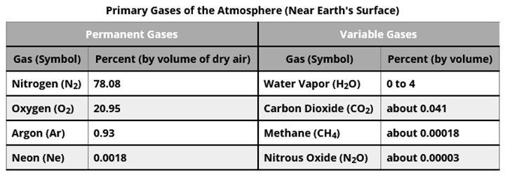
Source: Steve Seman, Penn State

As the chart above shows, the dominant atmospheric gases are nitrogen and oxygen, with argon a distant third. We are all familiar with the role of oxygen in our lives and in the process of creating energy. Nitrogen has its own cycle that creates nitrates that are protein for plant life before recycling.

Water vapor is also important, which fluctuates over time. According to NASA, water vapor is the most important gas in the atmosphere. Water constantly cycles through the atmosphere as it evaporates from the Earth’s surface, rises on warm updrafts, and condenses into clouds, is blown by the wind and then falls back to Earth as rain or snow. This is one way in which heat is transferred from the surface to the atmosphere and transported from one place to another.

The key GHG are CO₂ and CH₄. CO₂ is emitted by burning carbon-rich fossil fuels. While it is not the most powerful GHG, it is the most plentiful. It lasts longer in the atmosphere than other GHG. It is part of the natural carbon cycle that moves carbon from the surface to the atmosphere, and it is also absorbed by oceans and organic matter. This is a key role for CO_2.

CH₄ has a minor presence in the atmosphere. It is about 25-times more powerful than CO₂, but it is resident in the atmosphere for only about 11 years, considerably shorter than for CO₂. It comes from the decomposition of plant matter, being released from landfills, swamps, rice paddies, and by volcanoes and subaqueous vents. CH₄ is also emitted through natural gas flaring, and leaks during production and transportation. Cattle are also a major source of CH₄.

Nitrous oxide comes from bacteria in soil and livestock waste management. Modern agricultural practices, such as the use of nitrogen-rich fertilizers can contribute to nitrous oxide emissions. While almost negligible in the atmosphere, a single molecule has 298-times the global warming potential of CO₂.

Other GHGs that can contribute to global warming include hydrofluorocarbons (1,430-14,800 times the global warming potential of CO₂) and sulfur hexafluoride (22,800 times the global warming potential of CO₂).

The following chart shows the relationship between CO₂ and temperature over a very long geological timescale. The purple line measures CO₂ from atmospheric, ice core and fossil sediments extending back for millions of years. As the line shows, CO₂ levels were historically low since the middle of the Pliocene era, which is at about the three-million-year mark. Since then, CO₂ levels were flat, only showing an uptick in very recent years, which is at the extreme right-hand side of the chart. The last time the planet’s CO₂ was at such a low point was during the Carboniferous, Permian, and Triassic eras. Otherwise, CO₂ levels have been substantially higher than now.

Exhibit 7. Geological Timescale: Concentration of CO₂ And Temperature Fluctuations

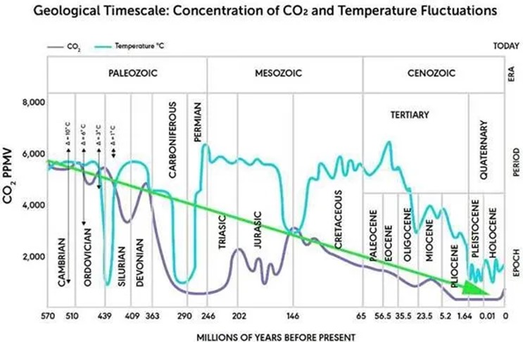
Source: Patrick Moore, Fake Invisible Catastrophes And Threats Of Doom

Patrick Moore, co-founder of Greenpeace, points to the geological history of the last 570 million years as key to understanding climate change, especially whether CO₂ is really the driver for hotter temperatures. He points to the 146-million-year mark in the chart above and commented: “carbon dioxide and temperature were 100 percent out of sync with each other for about 30 million years before the mark, and for about 100 million years after.” He also points out that there have been other long periods when these two factors moved in opposite directions. Those times include during the Silurian and Permian eras.

Moore’s point is that the simultaneous rise of CO₂ and temperatures for the past 170 years does not support a “strong cause-effect relationship.” He points out that the relationship between “correlation” and “causation” is subtle. Correlation that shows two factors closely related does not prove causation, while causation requires a strong correlation. Correlation may be caused by a third factor, often not clearly obvious. He cites the example of a high correlation between ice cream consumption and shark attacks. The third factor in this relationship is summer temperatures. In warm weather, people eat more ice cream, swim more, and suffer more shark attacks. This correlation doesn’t hold in winter months.

As mentioned earlier, the current rise in CO₂ is coming from an historical low level, only seen between 300 to 220 million years ago. What was interesting was finding a National Academy of Science paper by U.K. animal and plant scientist D. J. Beerling from the University of Sheffield titled “Low atmospheric CO₂ levels during the Permo-Carboniferous glaciation inferred from fossil lycopsids.” The paper’s abstract spells out the issue being examined and its significance for today’s climate.

Earth history was punctuated during the Permo-Carboniferous [300–250 million years (Myr) ago] by the longest and most severe glaciation of the entire Phanerozoic Eon. But significant uncertainty surrounds the concentration of CO2 in the atmosphere through this time interval and therefore its role in the evolution of this major prePleistocene glaciation. Here, I derive 24 Late Paleozoic CO2 estimates from the fossil cuticle record of arborsecent lycopsids of the equatorial Carboniferous and Permian swamp communities. Quantitative calibration of Late Carboniferous (330–300 Myr ago) and Permian (270–260 Myr ago) lycopsid stomatal indices yield average atmospheric CO2 concentrations of 344 ppm and 313 ppm, respectively. The reconstructions show a high degree of self-consistency and a degree of precision an order of magnitude greater than other approaches. Low CO2 levels during the Permo-Carboniferous glaciation are in agreement with glaciological evidence for the presence of continental ice and coupled models of climate and ice-sheet growth on Pangea. Moreover, the Permian data indicate atmospheric CO2 levels were low 260 Myr ago, by which time continental deglaciation was already underway. Positive biotic feedbacks on climate, and geotectonic events, therefore are implicated as mechanisms underlying deglaciation.

Let’s see if we can decipher the study. We know that glaciers covered much of the world at various points in the past. In fact, it is estimated there were at least eight glacial cycles during the last 740,000 years alone. As the glaciers advanced and retreated, they reshaped the landscape. According to Internet Geography, the Ice Age in the U.K. lasted from about one million years ago to about 20,000 years ago. Throughout that time, the northern and eastern parts of the British Isles were covered in ice. In some places, the ice was three kilometers (1.9 miles) thick. The article points out that the Lake District in the U.K. was carved out by the last glacier. Glaciation is the study of ice and its impact on the environment. But understanding the forces that trigger an ice age and its ending are important for assessing climate cycles.

Another term in the abstract many people may not be familiar with is Pangea. This was a supercontinent during the Late Paleozoic and early Mesozoic eras. It was assembled from earlier continents approximately 335 million years ago and began to break apart about 175 million years ago. Pangea was centered on the Equator, in contrast to the present Earth where continents are distributed around the world. Pangea was the first supercontinent to be reconstructed by geologists and provides scientists with the ability to match sediments from various continents that were originally all part of one.

Exhibit 8. Map Of Geologists Recreation Of Pangea Continent

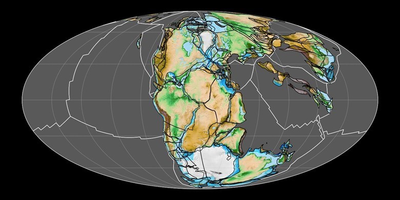
Source: Fama Clamosa – Own work, https://commons.wikimedia.org/w/index.php?curid=85466018

How is the analysis comparing temperatures with CO₂ and CH₄ conducted? Instrument measurements are key for the near-term, but for longer histories, studying analyses of ice cores and the sediments of fossils found in soil are the primary tools. When the text above refers to lycopsids, it is referencing herbaceous vascular plants, which are green, leafy plants with no woody structure. Members of this class of plants are clubmosses, firmosses and quillworts. When the botanists examine the fossilized remains of these plants, they are focused on the stomate, which is the minute pores in the epidermis of a leaf through which gases and water vapor pass. Examining the diameter of these pores, scientists can attempt to assess how the plants were reacting to the temperatures and concentration of CO₂ and CH₄ in the atmosphere.

As the abstract states, low CO₂ levels during the glaciation period were consistent with other glaciation evidence (fossil sediments) of ice and match the computer models of climate and ice-sheet growth. What the author of this paper concluded was that the level of CO₂ in this era was at the low end of the range of estimates from other sediment studies. More importantly, these low-level estimates (in red) in the bottom half the chart below are consistent with the low CO₂ levels shown from various periods during the Devonian, Carboniferous, and Permian eras (shown in purple in the preceding chart). What we have confirmed is that the low levels of CO₂ we had been experiencing, albeit today’s levels are higher than the most recent lows, are consistent with the low levels seen in prior glaciation periods.

Exhibit 9. Confirming Record Low CO₂ Levels In Climate History

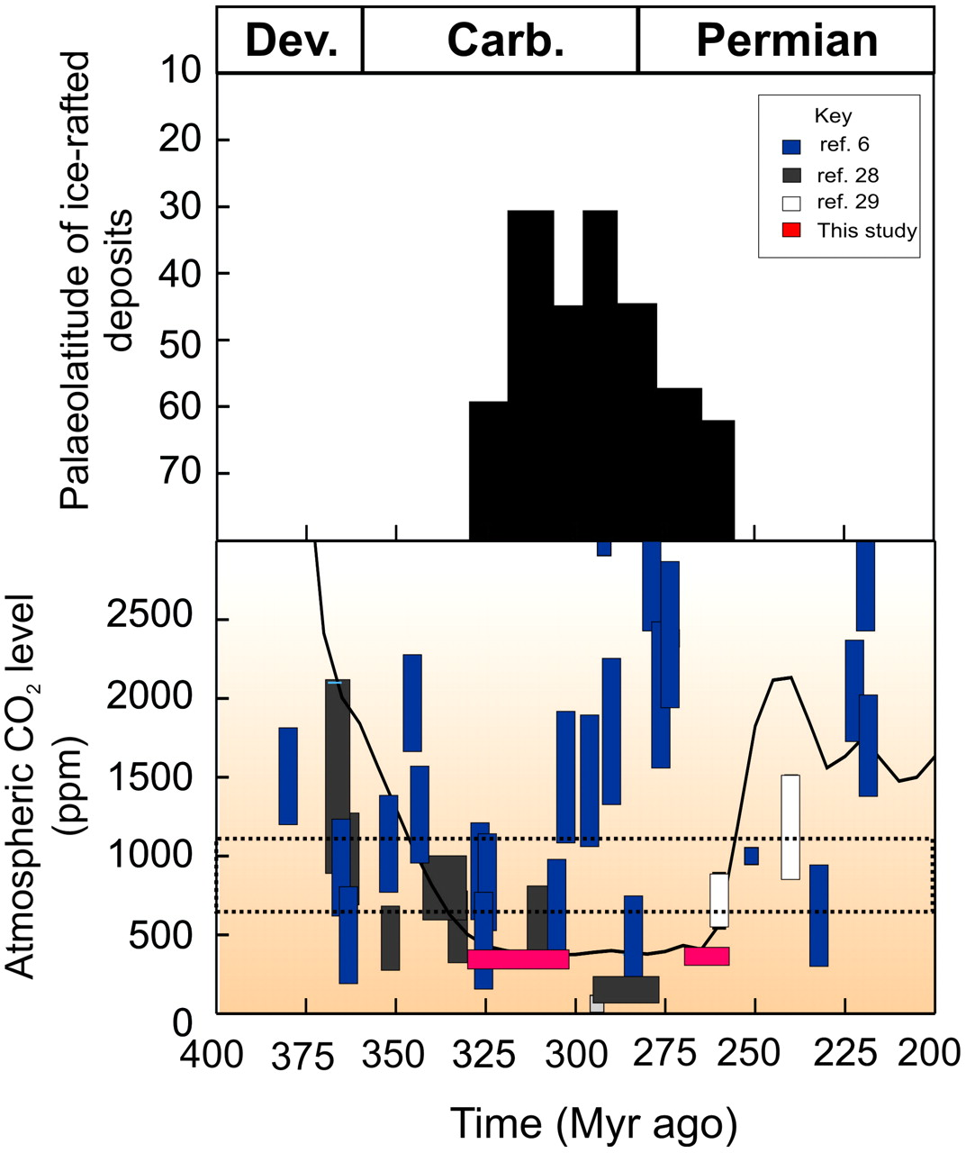
Source: D. J. Beerling

The Vostok ice core has been studied by many scientists and their reports published by numerous scientific publications. Highly respected geologist Euan Mearns, who writes a blog at Energy Matters, wrote two articles assessing the ice core’s data and explaining his view of the relationship between CO₂ and temperature, as well as how the relationship changed depending on the state of glaciation. The first article appeared in 2014 but was ignored by most climate scientists. He revisited the ice core topic in an expanded article in 2017.

The research and his first article were criticized, which is par for the course in the world of climate science research. We found Mearns’ research of value, but the critics views are also worthy. What these contrary positions yield is confirmation that the science is not settled and, in fact, the nature of the criticism of Mearns’ research gradually shifted away from the conventional view of climate change dynamics, as the comment thread stretched over two years and new research emerged.

 

As previously mentioned, there have been eight glacial cycles in the ice core. That provides significant data for study, particularly how the temperature, CO₂, and CH₄ relationships shifted as the cycles move from the inception of glaciation to its termination. In his article, Mearns produced a plot of the temperature and CO₂ drawn from the data reported for the Vostok ice core. His chart showed the most recent data displayed going from left to right, with the far right representing the oldest data. This is the opposite of what we are accustomed to seeing when we look at data displayed over time. The most recent data is for 1995, the year the ice core was drilled. Mearns also used the same data scales as employed in the seminal paper on the Vostok ice core, to avoid controversy over the graph’s presentation.

Exhibit 10. Vostok Ice Core CO₂ And Temperature Data

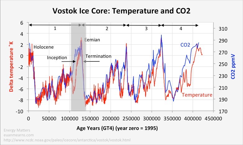
Source: Energy Matters

In Mearns 2014 article, he concluded that the lag between temperature and CO₂ was 8,000 years. That lag expanded to 14,000 years in the 2017 paper. The opening paragraph of the 2014 article sets out the issue Mearns explores and his conclusion. He wrote:

In their seminal paper on the Vostok Ice Core, Petit et al (1999) note that CO₂ lags temperature during the onset of glaciations by several thousand years but offer no explanation. They also observe that CH₄ and CO₂ are not perfectly aligned with each other but offer no explanation. The significance of these observations [is] therefore ignored. At the onset of glaciations temperature drops to glacial values before CO₂ begins to fall suggesting that CO₂ has little influence on temperature modulation at these times.

Shown below is the chart of the ice core’s temperature record compared with that of CH₄.

Exhibit 11. Measuring Temperatures and CH₄ In The Ice Core

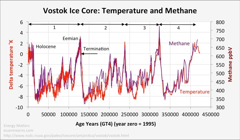
Source: Energy Matters

As Mearns points out, the fit of CO₂ to temperatures is not as tight as for CH₄. There is a tendency for CO₂ to lag temperature throughout the time series, with the time lag being most pronounced at the onset of each glacial cycle “where CO₂ lags temperature by several thousand years,” according to the paper by Petit et al. Mearns went on to examine other relationships that might explain why the lags exist between CO₂ and CH₄ and temperatures. These included the ice sheets and thawing of permafrost.

To demonstrate the relationship of CO₂ and CH₄, Mearns posted the following chart showing how the two gases moved together over the ice core history.

Exhibit 12. Movement Of CO₂ And CH₄ In Vostok Ice Core History

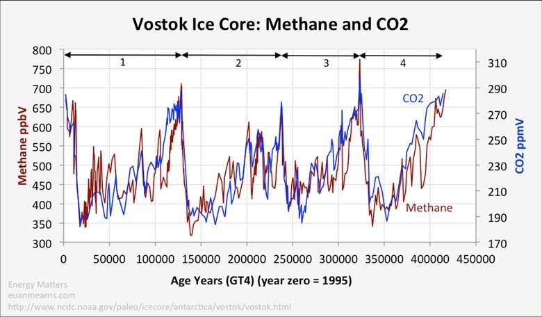
Source: Energy Matters

Mearns stated his conclusions thusly:

• Over four glacial cycles CO₂, CH₄ and temperature display cyclical co-variation. This has been used by the climate science community as evidence for amplification of orbital forcing via greenhouse gas feedbacks.
• I am not the first to observe that CO₂ lags temperature in Vostok and indeed Petit et al make the observation that at the onset of glaciation CO₂ lags temperature by several thousand years. But they fail to discuss this and the fairly profound implications it has.
• Temperature and CH₄ are extremely tightly correlated with no time lags. Thus, while CO₂ and CH₄ are correlated with temperature in a general sense, in detail their response to global geochemical cycles [is] different. Again Petit et al make the observation but fail to discuss it.
• At the onset of the last glaciation the time lag was 8,000 years and the world was cast into the depths of an ice age with CO₂ variance evidently contributing little to the large fall in temperature.
• The only conclusion possible from Vostok is that variations in CO₂ and CH₄ are both caused by global temperature change and freeze thaw cycles at high latitudes. These natural geochemical cycles makes it inevitable that CO₂ and CH₄ will correlate with temperature. It is therefore totally invalid to use this relationship as evidence for CO₂ forcing of climate, especially since during the onset of glaciations, there is no correlation at all.

Although the first article had 8,000 reads, Mearns was frustrated by the lack of attention paid to it by climate scientists. He believed his analysis raised serious questions that climate scientists should have commented on. That appears to be the rationale for his 2017 article. In a criticism of the 2017 article and Mearns mentioning the viewership and lack of climate scientists’ interest, a critic suggested maybe Mearns’ view of its significance wasn’t so profound.

Mearns wrote in the 2017 article that he planned to address the issue of the time lag. His article begins with:

Time lags of a few hundred years can be explained by dating errors and calibrating the gas ages to the ice ages (see my earlier post). This has caught the attention of the climate science community and for example Parrenin et al (2013) revised the gas ages in Vostok over the time interval 10,000 to 22,000 years ago that spans the termination that preceded the Holocene interglacial where the established chronology already showed good alignment between CO₂ and T (temperature). Parrenin et al conveniently forgot to examine the relationship at the inception where the time lag of several thousand years is so large, it is not possible to explain it by a calibration error.

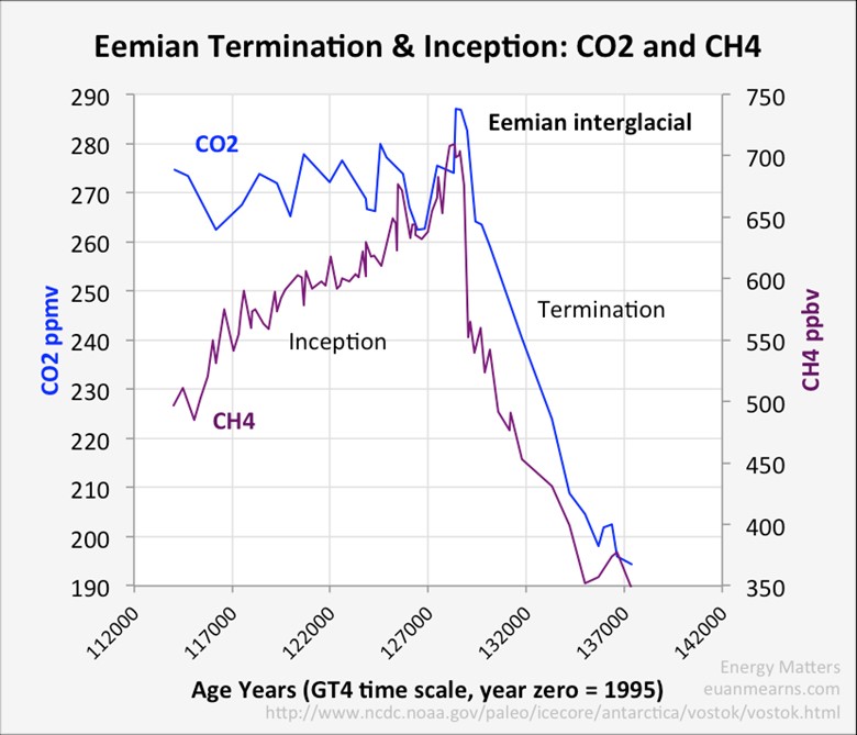
The subject of this post, therefore, is to look closely into the relationship between T, CO₂ and CH₄ in a narrow time band that spans the pre-Eemian termination and post-Eemian inception.

Mearns went on in his article to lay out the relationship between temperature and CO₂ over the years covering the inception of the post-Eemian glaciation era and the termination of the Eemain glaciation era. He does this through a series of charts that showed the data with explanations. He later augmented the analysis by extending the data timeline (Exhibit 15, page 20).

The period of 128,300 to 114,082 was selected for analysis because it marked the period when CO₂ went sideways. The chart shows that over 14,218 years, CO₂ did not change while temperature dropped by 7.23º K (Kelvin).

Exhibit 13. How CO₂ And Temperature Moved At Eemian Glacial Inception

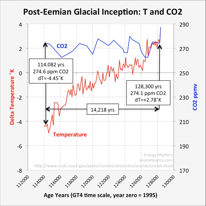
Source: Energy Matters

Before expanding the time of the data analyzed, Mearns introduced a chart showing the relationship between CH₄ and temperature to demonstrate how closely these two measures fit. If one compares the early years of the analysis (128,300 forward), there was a close fit between temperature and CO₂ (Exhibit 13), but certainly not with CH₄ (Exhibit 14). That relationship changed at about 126,000 years ago when CH₄ began to closely track the downward movement in temperature while CO₂ remained flat.

Exhibit 14. How CH₄ And Temperatures Moved In Post-Eemian Ice Age

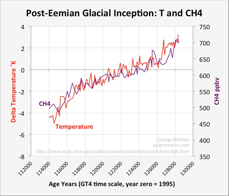
Source: Energy Matters

By extending the time-period studied, Mearns discovered additional perspective. He extended the time by 12,253 years to 101,829 years ago. He separated his analysis into three parts. The first showed how temperatures fell from the Eemian peak to the point where CO₂ stopped going sideways. The second phase showed temperature falling to a low of -7º K at 108,000 years ago. Phase three showed an interesting development. Temperature rebounds while CO₂ goes sideways once again. In Mearns view, this shows that CO₂ has little to do with modulating temperatures during glacial cycles.

Exhibit 15. Extending The CO₂ And Temperature Data During Eemian Ice Age

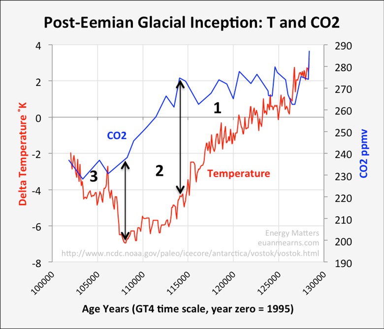
Source: Energy Matters

The next step in the analysis was to expand the time frame analyzed to include the termination phase – further into the past. Termination is when the glaciation ends, and large Northern Hemisphere ice sheets collapse and melt. During this period, temperature and CO₂ are closely linked. As the oceans warmed, they released trapped CO₂. This is important, as we have already seen that the oceans did not absorb and bury CO₂ until 14,000 years had passed. Temperature and CH₄ are not as closely linked in this period, although they rise together with a time lag of a few thousand years.

Exhibit 16. How CO₂ And Temperatures Moved During Eemian Glacial Era

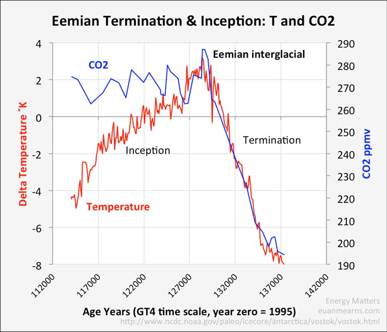
Source: Energy Matters

Exhibit 17. How CH₄ And Temperatures Moved During Eemian Glacial Period

Source: Energy Matters

To better illustrate the difference between CO₂ and CH₄, Mearns plotted the concentrations of the two gases over the inception and termination of Eemian glaciation.

Exhibit 18. Divergence In Trend Of CO₂ And CH₄ In Vostok Ice Core

Source: Energy Matters

Before launching into a discussion of speculative explanations for the movement of the carbon gases and temperature in the Vostok ice core, Mearns made the following observations.

1. CO₂ and temperature are closely coupled at the glacial termination, both rising together.
2. CH₄ and temperature are less well coupled at the glacial termination, CH₄ rising up to 2,000 years after temperature.
3. CO₂ is decoupled from temperature at the glacial inception remaining constant for over 14,000 years while temperatures plunge over 7˚K.
4. CH₄ is closely coupled with temperature at the glacial inception, both falling together.
5. At the onset of the glacial termination 137,341 years ago, albedo is high owing to extensive ice sheets but the next thing to happen is that temperatures rise.
6. At the onset of the glacial inception 128,357 years ago, on the peak of the Eemian interglacial, albedo is low but the next thing to happen is that temperatures fall.
7. Variations in CO₂ and CH₄ need to be explained by bio-geochemical processes combined with temperature variations and changing land and sea ice cover.
8. CO₂ and CH₄ are responding in different ways to events and therefore have different sources and sinks.
9. The overall pattern of glacial cycles are controlled by Milankovitch orbital cycles, but these alone are too weak to account for the large temperature fluctuations.

Albedo refers to the fraction of incident radiation (such as light) that is reflected by a surface or body (such as the moon or a cloud).

We thought it was appropriate to show a slightly different chart of temperature versus CO₂ for the time-period Mearns focused on. This scale and layout may make it easier for readers to track how CO₂ lags temperature changes, although there are several brief periods when the two metrics coincide. That becomes the CO₂ conundrum.

Exhibit 19. Vostok Ice Core Shows Lad Between Temperatures And CO₂

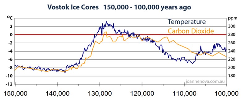
Source: joannenova.com.au

After presenting all his observations and preliminary conclusions, Mearns wrestles with what forces might be triggering the glaciation and deglaciation eras if they are not CO₂ or CH₄. His conclusion is the only two forces strong enough to trigger these changes would be the Sun or the oceans. The Sun has played a role in climate studies for a long time and continues to play a role. So too have the oceans. They are known to be a way of transferring heat from one part of the world to another. The mechanism is known as the Atlantic Multi-decadal Oscillation (AMO). The cycle has an estimated period of 60-80 years. It is based on the average anomalies of sea surface temperatures (SST) in the North Atlantic basin.

The observed AMO index, defined as the detrended 10-year low-pass filtered annual mean area-averaged SST anomalies over the North American basin is shown in the chart below. The chart shows the positive (warm) and negative (cool) periods of the AMO compared to the 5-year annual average of tropical cyclone activity.

Exhibit 20. The Pattern Of Atlantic Ocean Multi-decadal Oscillation Over 145 Years

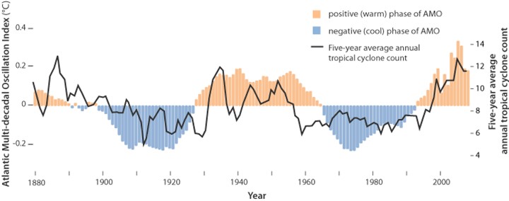
Source: energyeducation.ca

Mearns’ theory to explain the glaciation changes is the simple idea that the circulation of the modern era is a function of the natural world and depends upon the delicate climate balance that cycles ocean water from the tropics toward the poles and back again, allowing heat to be dissipated and CO₂ to be absorbed and disgorged. In the Northern Hemisphere, the cycle is driven by warmer water moving northward, which then experiences evaporation that increases its salinity as it arrives in the north, which contributes to the formation of sea ice further increasing the water’s salinity. The cooler saline water sinks and flows along the ocean floor back to the tropics where it warms and the cycle restarts.

The evidence suggests that the earth’s tilt (obliquity) can upset this delicate climate balance causing the cycle to either shut down or to begin. This point leads to questioning whether, as Mearns suggests, the Sun may be playing a role in our rising temperatures. A century ago, Serbian scientist Milutin Milankovitch hypothesized the long-term, collective effects of changes in Earth’s position relative to the Sun being a strong driver of Earth’s long-term climate and may have been responsible for triggering the beginning and ending of glacial periods.

Through research, he developed and calculated the duration of three cycles. The Milankovitch cycles are:

• The shape of Earth’s orbit not being a perfect circle is known as eccentricity (~100,000 years).
• The angle the Earth’s axis is tilted with respect to its orbital plane is known as obliquity (~41,000 years).
• The direction the Earth’s axis of rotation is pointed is known as precession (~26,000 years). The slow rotation or “wobble” in the Earth’s axis of rotation changes the annual orbital path of the Northern Hemisphere summer solstice occurs.

How do these cycles work, and what is their potential impact on Earth’s climate?

With respect to eccentricity, when the Earth’s orbit is at its most elliptic, about 23% more solar radiation reaches the planet when it approaches closest to the Sun each year than it does at its farthest point away. The variations in the Earth’s eccentricity are fairly small, so they only play a minor factor in annual season climate variations.

Obliquity impacts the magnitude of cooling and warming experienced. When obliquity decreases, it gradually makes our winters warmer and summers cooler. Over time, this enables snow and ice at high latitudes to build up into large ice sheets. As the ice cover grows, it reflects more of the Sun’s energy back into space, promoting even further cooling.

Precession, or “wobble” is caused by tidal forces impacted by gravitational influences of the Sun and Moon that cause the Earth to bulge at the equator, affecting its rotation. The trend in the direction of the wobble relative to the fixed positions of stars is known as axial procession. There is also apsidal precession, in which the Earth’s entire orbital ellipse also wobbles irregularly, primarily due to the shifting mass as ice cover melts.

The research has shown these cycles to exist, but their impact on climate is over extremely long durations of time – tens of thousands of years. These cycles do not play much of a role in explaining our current warming. What does? CO₂ and CH₄ are important, and a key to how they may influence temperature changes is ocean circulation.

For the past 1.2 million years, there has been more resistance to ocean circulation being triggered and the glaciations have become substantially longer in duration. The changes in ocean currents also impact the patterns of atmospheric circulation leading to greater convection rates and increased cloud cover. Both forces can contribute to rapid cooling and warming. Mearns suggests that “during the glacial episodes we would not recognize the distribution of pressure systems as belonging to the Earth we know today. CO₂ in the past played a negligible role. It simply responded to bio-geochemical process caused by changing temperature and ice cover.” In other words, climate science is much more complex than many acknowledge and maybe we still don’t know exactly what moves temperatures.

We read criticism of Mearns articles by the web site “…and Then There’s Physics” authored by Ken Rice, Professor of Computational Astrophysics at the Institute for Astronomy at University of Edinburgh. Rice acknowledges he is not a climate scientist but is a scientist and involved in teaching science.

In Rice’s critique, he says:

Firstly, this is data from a single site (Vostok). Even though greenhouse gases may be well-mixed, the temperature is not. You need to be a little careful when using this single site to infer something about global temperatures, and the relationship between temperature changes and CO₂/CH₄ changes.

He went on to say:

It is certainly not the case that CO₂ is the main driver of the glacial cycles. The trigger for the glacial cycles is probably orbital variations, in particular large changes in solar insolation at high northern latitudes. However, the net change in solar insolation (globally) is small, so it cannot – by itself – produce much in the way of warming/cooling. What is thought to happen is that these changes trigger either ice sheet retreat, or ice sheet advance (depending on whether we’re moving into a glacial, or out of a glacial). This changes the planetary albedo which produces either warming (ice sheet retreat) or cooling (ice sheet advance).

This warming/cooling then results in the release/uptake of CO₂ from the oceans, and influences vegetation (which itself produces an albedo change and releases, or takes up, CO₂). The change in atmospheric CO₂ (and CH₄) then produces more warming/cooling, causes further retreat/advance of the ice sheets, and further changes in vegetation. These different processes (albedo changes and changes in atmospheric CO₂/CH₄) then together produce the temperature changes that move us into, or out of, a glacial period.

What this critique suggests is that Mearns speculation about how other forces than CO₂ and CH₄ are driving the initiation and termination of glacial ages is probably correct. When you read Rice’s writings and the papers cited to augment his argument, you are left to conclude that ocean circulation is key to climate change dynamics. Importantly, Rice concludes that CO₂ is not a forcing in the climate but a feedback factor.

A new peer-reviewed paper addresses the recent science of the Vostok ice core and the linkage and roles of CO_2, CH₄, and temperatures in explaining climate change. It was published in May 2021 but was challenged in June for its peer-review process, which we will address in a later article. The paper, “The temperature–CO₂ climate connection: an epistemological reappraisal of ice-core messages” was authored by Pascal Richet of the Institut de Physique du Globe de Paris and published by History of Geo-and Space Sciences.

At the heart of the paper, the author questions why climate models that cannot account for the lag in temperature and CO₂ in the past are accepted for explaining our future global climate. He shows how throughout science history, well established and believed scientific theories about the world were overturned with new data and explanations. In some cases, theories were believed, rejected, but later re-accepted when scientific investigations progressed and produced new data. That part of the paper is a fascinating read about the history of science and famous scientific theories and their authors.

Richet focuses on the relationship between changes in temperature and the level of CO₂ over the past four glacial cycles in Antarctica. He observed:

The fact that the peak widths are systematically larger for CO₂ than for temperature thus implies that the variations in CO₂ concentrations were driven by temperature changes throughout all cycles and not only at their onsets. Of particular interest in this respect are the peaks signaled by one or two solid dots in [the top chart below]. Because, in each instance, a single CO₂ peak correlates with a temperature doublet, such features would again plainly violate the non-contradiction principle if variations in CO₂ concentrations were considered as causes and temperature changes as effects.

Making physical sense of this conclusion is straightforward. The total amount of CO₂ in the atmosphere is only a tiny fraction of that present in the ocean (Lee et al., 2019). Even though the acid base properties of CO₂-bearing aqueous solutions and the biological role of carbonate and bicarbonate ions make the picture difficult to unravel quantitatively (see Michard, 2008), temperature rises cause an overall decrease in the CO₂ solubility in the ocean and, correlatively, an increasing concentration of atmospheric CO₂.

The chart Richet references is below. The four cycles range from 87,000 to 123,000 years in duration. The fifth cycle at the far right is very short. What we see for each cycle is a horizontal bar showing the duration of the peaks for CO₂ and temperature. In each cycle the duration of the CO₂ peak is longer than for the corresponding temperature. This is consistent with Mearns’ view.

Exhibit 21. CO₂ Takes Longer To Peak Than Temperatures Suggesting A Lag

Source: History of Geo-and Space Sciences

If CO₂ lags temperature changes by a significant number of years, then it is difficult to perceive it as a “forcing” agent, i.e., driver, of global warming. Of course, that is exactly what the IPCC in its AR6 report calls CO₂. From the Summary for Policymakers, we have the following statement on page 7:

A.1.3 The likely range of total human-caused global surface temperature increase from 1850–1900 to 2010–2019 is 0.8°C to 1.3°C, with a best estimate of 1.07°C. It is likely that well-mixed GHGs contributed a warming of 1.0°C to 2.0°C, other human drivers (principally aerosols) contributed a cooling of 0.0°C to 0.8°C, natural drivers changed global surface temperature by –0.1°C to 0.1°C, and internal variability changed it by –0.2°C to 0.2°C. It is very likely that well-mixed GHGs were the main driver of tropospheric warming since 1979, and extremely likely that human-caused stratospheric ozone depletion was the main driver of cooling of the lower stratosphere between 1979 and the mid-1990s. (emphasis added)

Rice and other critics of Mearns research acknowledge the CO₂-temperature lag seen in the Vostok ice core, but insist it is not important because CO₂ is not a “forcing” agent but a “feedback” factor.

We are left to wonder about the role of CO₂. If it is not the “forcing” agent the IPCC says, then what are we to make of the climate models that use CO₂ data and projections to drive them? These are the models the IPCC relies on to predict the dire climate outcomes they have been projecting for decades. What we believe is that CO₂ and CH₄ do function as feedback mechanisms in the climate system. As a feedback mechanism, it acts to disrupt the natural carbon cycle, and that is important. As Koonin stated:

So while carbon dioxide, in and of itself, is not particularly a concern for the planet, what is a concern is that, because life today has evolved to be well-suited to a low level of CO₂ (anatomically modern humans appeared only some 200,000 years ago…), the rapid increases of the past century might prove disruptive.

Koonin went on to explain that future climates will be determined by climate’s response to human, natural, and internal influences. Natural and internal factors include volcanoes, the Sun, and deep ocean currents. We can make assumptions about their impact on emissions and aerosols, but they are only that – assumptions. Human influences relate to our energy consumption patterns.

Future emissions from human activities will depend on future demographics, economic growth, regulations, and the energy and agricultural (largely related to CH₄ emissions) technologies in use. By making assumptions about each of these variables and their projected emissions, aerosol concentrations and changes in land use, we can develop a sense about how the climate might respond to human influences in the future. This is where Koonin suggests we should be wary of what the climate models project.

Koonin’s comments on climate models prefaced his discussion of the various pathway scenarios developed by the IPCC to highlight how future climates might unfold. Those scenarios will be addressed in a future Energy Musings. In the meantime, we believe it is important to read what Koonin wrote about the pitfalls policymakers may encounter by blindly accepting the worst of the scenarios as the “likely” outcome.

He wrote:

But it is here that the warning light should start blinking. Despite the certainty with which projections are reported as facts, estimating human influences is a highly uncertain business. Imagine being back in 1900 and trying to project what civilization would be like in the year 2000. At the time, the first powered flight and the first mass-produced automobile were yet to come, radio had just been invented and X-rays just discovered, and antibiotics weren’t even imagined. Even the most prescient prognosticator back then would have missed most of what transpired in the subsequent century as the global population quadrupled and the global economy grew by a factor of forty! They’d be amazed at the scale and rapidity with which people, goods, and information now move around the globe, at how we manufacture, and at our advances in agriculture and medicine.

None of what we have discussed about the long-term climate science and the more recent warming leads us to reject global change. Whether the planet continues warming on the same temperature trajectory as experienced over the past century is debatable. This is where the climate models come into play along with the roles of CO₂ and CH₄. The oceans also play a role in the carbon cycle, and potentially a more important role than we fully comprehend.

One conclusion we draw is that limiting CO₂ and CH₄ emissions is necessary. Due to their geochemical properties that promote warming once in the atmosphere, we must also acknowledge that warming will not stop immediately even if emissions go to zero. Eliminating emissions is a political problem that requires social, financial, and technological evaluations to be able to convince everyone to change how they live their lives today. What are the options, especially when one accepts the reality that zero emissions on the timetable demanded is not likely to happen?

As businessmen and generals have learned over the years, plans, forecasts, and models are wrong as soon as they are prepared. Their value is in the effort to develop them, which requires focusing on the forces that drive the future environment, but importantly also identifying those forces that we do not fully understand and how they might disrupt that future environment. This requires recognizing the uncertainty of the planning process and the need to be open to new data and interpretations of the data. As Winston Churchill put it: “Plans are of little importance, but planning is essential.” We agree.

EVs Are In The News But Not Always In The Best Light

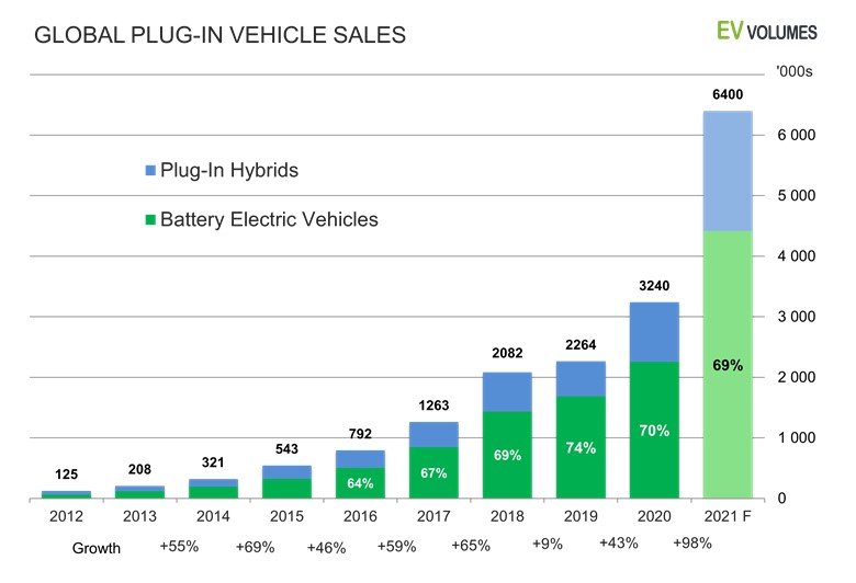
Electric vehicle (EV) sales were up strongly worldwide during the first half of 2021. Based on sales tracked by ev-volumnes.com, one of the top monitors of this market, 2.65 million new EVs were sold in 1H2021, an increase of 168% over last year. That growth was helped by comparing to a weak 1H2020 due to the pandemic. Compared to 1H2019, EV sales fell 14%. However, overall light-duty vehicle sales fell 28%. EV sales recovered in 2H2020, especially in Europe, as buyers prepared for the implementation of the 95 grams of CO₂ emissions mandate, as well as governments providing extensive green recovery funds. Other EV market monitors cited more new EV models helping to drive buyer interest.

Exhibit 22. EV Sales Are Going Very Well In 2021

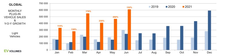
Source: ev-volumes.com

Articles about EVs tend to lump both battery EVs (BEV) and plug-in hybrid EVs (PHEV) together when discussing the market. For example, as ev-volumes.com points out, for all regions and most countries, EV sales grew 3%-8% during 1H2021. The EV share of global light-duty vehicle sales rose from 3% last year to 6.3% in 1H2021. Europe’s share doubled during this time to 14% from 7% in 2020. However, half of Europe’s EV sales are PHEVs, while outside of Europe the ratio is more like 20%.

As the chart below shows, PHEVs represented 31% of total EV sales in 1H2021. That is a greater share than in either 2019 or 2020, but equal to 2018’s share.

Exhibit 23. Global EV Market Has Large Share Of Hybrid EVs

Source: ev-volumes.com

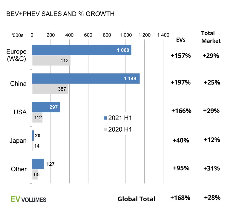
What is also significant is European and Chinese dominance in the global EV market. The U.S. has a meaningful presence, but it represents less than a third of those two dominant markets. The chart below highlights respective EV sales versus overall light-duty vehicle sales in each market. The global EV business, however, remains highly dependent on a few markets. That is because EV markets are driven by different forces. In Europe, it is due to green energy mandates calling for banning internal combustion engine (ICE) vehicles, plus healthy buyer subsidies. In China, air pollution in major cities has been a driver for EVs, but the government is promoting an industrial business strategy to dominate clean energy technology to match its dominance in rare earth minerals mining and processing, key to these technologies. Call it the Great Leap Forward in EVs, designed to mirror China’s successful corralling of the global solar panel market.

Exhibit 24. EV Sales And Fleet Are Significant In Three Global Markets

Source: ev-volumes.com

In the global effort to fight climate change, EVs play a key role. EVs enable countries to “electrify” their transportation sectors, major contributors to carbon emissions. With vehicles powered by electricity, the countries can push to revamp their power grids to use only green energy, further helping reduce emissions.

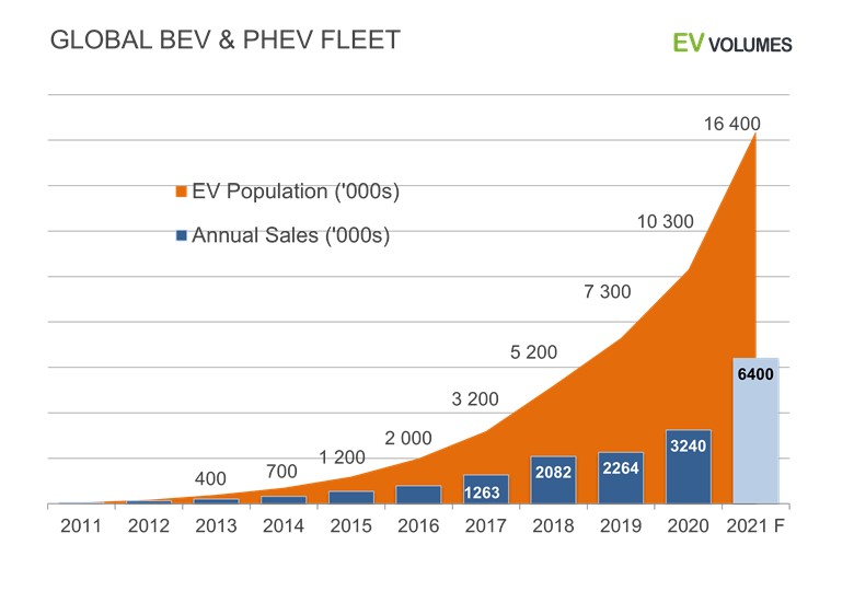
While the annual and cumulative sales are impressive, EVs’ share of the world’s light-duty vehicle fleet is small. The chart below assumes 6.4 million EVs are added to the global fleet in 2021, bringing EVs’ cumulative total to 16.4 million. That represents about 1.1% of the estimated 1.5 billion light-duty vehicles operating worldwide.

To demonstrate the challenge of electrifying the global light-duty vehicle fleet, ev-volumes.com offered a scenario (one of many) for EV fleet growth. They begin noting that the global light-duty fleet is growing by roughly 40 million units per year. In projecting EV sales to reach 100% of zero-emission light-duty vehicle sales in 2040, the global vehicle fleet grows to two billion, with over 40% being BEVs, but over 50% of the fleet still burning gasoline or diesel fuel. This shows how challenging it is for a zero-emission transportation fleet to be created. It is especially true when one realizes the average age of a car in the U.S. (likely worldwide, too) is over 12 years. That means a new car sold this year will only reach the average vehicle age in 2033, just seven years away from the 2040 target. The only way to realistically change this projection is government mandates outlawing ICE vehicles. It will make more countries look like Havana, Cuba.

Exhibit 25. Despite Strong Sales EVs Still Small Share Of Global Vehicle Fleet

Source: ev-volumes.com

A complicating consideration is the technology of EV batteries. This was demonstrated in General Motors’ (GM) recent recall of all its Chevy Bolt EVs. The Bolt was a newly designed EV to replace Chevy’s earlier EV model, Volt, that was a problem seller. The most recent recall was the third for the Bolt. This recall was for models from 2020 through 2022, along with a few 2019 models not involved in an earlier recall. It involves 73,000 vehicles, 60,000 of which are in the U.S. A month earlier, GM recalled its 2017-2019 Bolts. That recall involved 68,000 vehicles, of which 51,000 are in the U.S. The earlier recall was estimated to cost GM $800 million, with the recent recall adding an additional $1 billion to the tab.

All the recalls are related to battery fires. At the time of the first recall, GM instructed Bolt owners to not recharge without being present, as well as to not park their vehicles in enclosed locations. Sam Abuelsamid, lead auto analyst for research firm Guidehouse Insights, said there had been seven Bolt fires, or about 0.006 percent of those on the road. GM has acknowledged 10 fires. He contrasted that with data from the National Fire Protection Association that said 212,000 gas and diesel vehicles caught fire in 2018, or about 0.07 percent of those on U.S. roads. The ICE vehicles catching fire likely suffered equipment malfunctions or driver errors, but the Bolt fires arise from unknown causes. Additionally, extinguishing EV fires is much more challenging and water intensive. The bigger problem is that EVs and their batteries represent “new” technologies auto companies are investing tens of billions of dollars in to revamp their product lines. A black eye for the technology adds another challenge to getting people to purchase EVs.

The Bolt recall has created a battle between GM and its battery supplier, LG Chem, over who is at fault. GM obviously would like to shift the blame to LG Chem, making it responsible for the recall expense, which involves replacing the batteries of the Bolts. The recall expense represents a financial challenge for GM who is investing $35 billion in EVs between 2020 and 2025.

We are not surprised that GM wants to shift the blame, and the cost, to LG Chem. We estimate the recall cost per Bolt is $12,766. The high recall cost reflects the requirement to replace battery packs, the most expensive component of an EV. When we add to the recall cost the $10,000 per EV loss GM executives have stated, the “investment” in each Bolt increases to $22,766.

According to a February 2021 article by Green Car Report, with GM introducing two new EVs in 2022 – the $112,595 Hummer EV Edition and the expected nearly $60,000 Lyriq – it was faced with not having a more affordable offering. GM announced a $5,500 price cut for the 2022 Bolt, which was an adjustment to reflect the vehicle no longer being eligible for the $7,500 federal tax credit the company assumed its buyers would be get. By cutting the suggested retail price, GM was bringing the price down to $31,995, including the destination charge, for the Bolt EV and $33,995 for the Bolt EUV, a 6-inch longer model. The recall cost equals 38%-40% of the base cost, and if we add in the presumed $10,000 per unit loss, the financial impact climbs to 67%-71%. Currently, GM has stopped building Bolts. Not only is the recall a significant blow to Bolt’s profitability, but it becomes a reputational issue for GM at a critical point in the evolution of its business strategy, with potential long-term financial repercussions. Its low-end EV product, and only EV product, now has a questionable pedigree.

The bigger question about EVs is the religious belief that they are the cleanest alternative available. That belief rests on EVs not having tailpipes emitting pollution. It ignores the legacy carbon emissions involved in their construction, besides emissions from the power used to charge the battery. A new paper published on the techcrunch.com website, titled: “The tough calculus of emissions and the future of EVs” by Mark Mills, provides an in-depth assessment of the challenge in determining the carbon embodied in an EV. Mills, self-described as “Physicist, columnist, author, entrepreneur, board director, with a unique and innovative perspective on big trends in technology, markets, and policy, and on businesses realities,” explores this complex issue with substantive data that demonstrates how little is known about the issue, but importantly, what has not been considered is seeking an answer.

As Mills frames the discussion:

The issue is not primarily about the emissions resulting from producing electricity. Instead, it’s what we know and don’t know about what happens before an EV is delivered to a customer, namely, the “embodied” emissions arising from the labyrinthine supply chains to obtain and process all the materials needed to fabricate batteries.

We know virtually everything about the energy and emissions of ICE vehicles. We know very little about those issues for EVs.

For example, one review of 50 academic studies found estimates for embodied emissions to fabricate a single EV battery ranged from a low of about eight tons to as high as 20 tons of CO₂. Another recent technical analysis put the range at about four to 14 tons. The high end of those ranges is nearly as much CO₂ as is produced by the lifetime of fuel burned by an efficient conventional car. Again, that’s before the EV is delivered to a customer and driven its first mile.

To answer the question about embodied carbon emissions, Mills explores the chemistry of batteries and the materials needed to build them. He draws on the International Energy Agency’s (IEA) recent report on “transition energy minerals,” better known as rare earth minerals, which are employed in batteries. He examines the costs to extract, process and ship them to battery manufacturers. Given the weight of EV batteries, he examines the materials car builders use to make the vehicle lighter, but which adds to its embodied emissions total. In the future, these materials will need to be “clean,” adding further to the vehicle’s cost. These new materials and battery chemistries are years away from being proven and certainly from becoming mainstream, so the hopes for cleaner EVs are way out on the horizon. Mills concludes his paper by offering a radical solution –the cleaner ICE vehicles that already exist. He writes:

For policymakers eager to reduce automotive oil use, engineers have already invented an easier and more certain way to achieve that goal while awaiting revolutions in battery chemistry and mining. Commercially viable combustion engines already exist that can cut fuel use by as much as 50%. Capturing just half that potential by providing incentives for consumers to purchase more efficient engines would be cheaper, faster—and transparently verifiable—than adding 300 million EVs to the world’s roads.

When we consider Mills’ investigation of embodied carbon in EVs, the IEA’s prognosis of higher costs for rare earth minerals and other materials used in EVs, and the challenge of securing efficiencies and technological breakthroughs, coupled with the financial challenges of EVs for auto manufacturers, all the hoopla over recent global EV sales figures makes us wonder if anyone will suggest a timeout to reassess the road we are heading down?

Fossil Fuels’ Death Prediction May Be Premature

Given the Intergovernmental Panel on Climate Change’s (IPCC) recent report on our climate, we are not surprised the rhetoric for ending the burning of fossil fuels has ramped up. That rhetoric and demands for the death of fossil fuels will grow as we near the October 31 start of the 26th UN Climate Change Conference of the Parties (COP26). However, as we assess the global energy landscape, we find that past government climate policies and an uncooperative nature have led to a revival of fossil fuels use. A primary reason for the revival is the strong rebound in global electricity demand in 1H2021 in response to the economic recovery.

According to a report by Ember, a Community Interest Company in the U.K. that focuses on climate change and transitioning the grid, global electricity demand grew 5% in 1H2021 compared to 2019. The estimate comes from examining the data from 63 countries accounting for 87% of global electricity demand. The report estimates that 57% of the increased electricity demand was met by wind and solar, with the remainder coming from increased coal generation. The report also found emissions from the power sector increased 5% compared to 2019. Most of the increased electric demand and coal usage was in Asia, but Germany also contributed.

Exhibit 26. How And Where Emissions Have Risen In 1H2021’s Economic Recovery

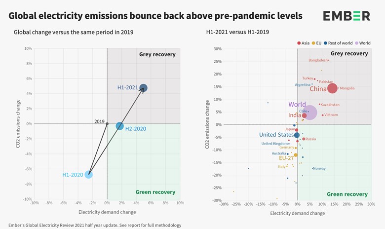
Source: Ember

With Germany’s economy rebounding strongly in 1H2021, the country’s power needs jumped. It occurred at the same time onshore wind output plummeted by more than 25%. Offshore wind was also down 16%. The share of renewable energy in Germany’s gross electric power consumption slumped in 1H2021 to 43% from 50% the prior year. Coal output increased 39% this year to meet the power demand.

Germany’s reduction of its coal-fired power lasted just eight days in January, after which its four largest plants needed to be restarted and operated in spinning mode to provide power whenever the grid frequency dipped. These plants now are seeking government subsidies to offset their high operating expenses relative to the little income generated when operating as peaking plants. Previously, these power plants consistently produced the country’s cheapest electricity without subsidies. The impact of these electric power market issues has Germans paying the highest residential electricity prices in Europe.

Exhibit 27. The Push For Clean Energy In Europe Is Driving Electricity Prices Up

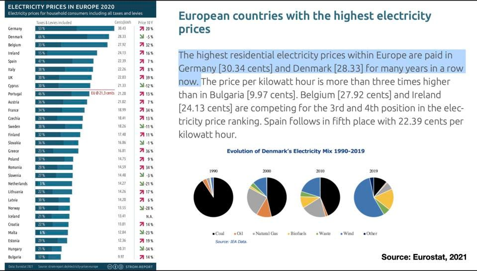
Source: Michael Shellenberger

In California, another high-cost electricity market, Governor Gavin Newsom (D) declared a state of emergency for its power grid last month over concern about supply shortages during hot summer evenings when solar output declines. Owners of electric vehicles were told to not recharge them during the 4-9 pm time slot to ease the demand. Air-quality rules were also waved to help ease the power crunch.

Last week, the California Department of Water Resources began securing five gas-fueled generators with capacities of 30 megawatts to provide additional power supply. The units are to be installed at existing power plants and should be operational by mid-September. These gas generators are called temporary, but they were issued 5-year operating permits. The irony is that earlier this year, California regulators balked at ordering utilities to add new gas-fired generation after being criticized by environmentalists over the effort running counter to the state’s plan for a decarbonized grid by 2045. Keeping the lights on seems to overrule environmental concerns.

Back in Europe, natural gas storage volumes are at their lowest levels in years as the injection season approaches its end. Gas prices are soaring, forcing utilities to restart coal plants due to their power being consistent and cheaper. Because lignite is often used, CO₂ emissions are rising, as it is the dirtiest coal available. Europe’s challenge is getting more gas from Russia, whose capacity to supply the continent will expand once the Nord Stream 2 pipeline becomes operational. Although there are only 10 miles of pipe left to be installed, the pipeline will still require technical certification that takes time. However, even when the pipeline begins operations, Gazprom has not increased its gas production yet, therefore, initial supplies going through the pipeline will come from other pipelines supplying Europe. In other words, there is limited additional gas supply available. Europe can battle with Asia for additional liquefied natural gas (LNG) supplies, but few additional cargoes have headed there, as prices are soaring.

China has recently announced plans for more coal-fired power plants that flies in the face of pressure from environmentalists. According to a report from Greenpeace, Chinese provinces are planning to build more than 100 gigawatts (GW) of new coal-fired power plants despite a decline in new plant approvals in 1H2021. During the first six months of 2021, Greenpeace reported that local government agencies approved 24 new coal-fired power plants with a total capacity of 5.2 GW.

Last year, as the pandemic was raging across the world and governments were locking down economies, the plea was for governments to rebuild green. The recovery was perceived as an excellent opportunity for governments to pour billions into rebuilding but emphasizing clean energy as the foundation. This move was seen as an opportunity to move to kill off fossil fuels. These efforts appear to have failed as coal and natural gas demand is up strongly in 2021. Environmentalists are lamenting the Build Back Dirty outcome.

Contact PPHB:
1885 St. James Place, Suite 900
Houston, Texas 77056
Main Tel: (713) 621-8100
Main Fax: (713) 621-8166
www.pphb.com

Leveraging deep industry knowledge and experience, since its formation in 2003, PPHB has advised on more than 150 transactions exceeding $10 Billion in total value. PPHB advises in mergers & acquisitions, both sell-side and buy-side, raises institutional private equity and debt and offers debt and restructuring advisory services. The firm provides clients with proven investment banking partners, committed to the industry, and committed to success.